Project 1: Depolarizing channel

In this project we will implement the depolarizing channel in Qiskit and test it with state tomography on a simulator and optionally on a real device.

The depolarizing channel is one of the most common models of qubit decoherence due to its nice symmetry properties. We can describe it by stating that, with probability $1-p$ the qubit remains intact, while with probability $p$ an error occurs. The error can be a bit flip error, described by the action of $\sigma_x$, a phase flip error, described by the action of $\sigma_z$, or both, described by the action of $\sigma_y$. The dynamical map of a Markovian open quantum system subjected to depolarizing noise can be written as

\begin{align} \Phi_t \rho_S = \left[1-\frac 3 4 p(t)\right] \rho_S + \frac{p(t)}{4} \sum_i \sigma_i \rho_S \sigma_i, \end{align}

where $i=x,y,z$ and $p(t)=1 - e^{-\gamma t}$, with $\gamma$ the Markovian decay rate.

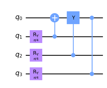
The depolarizing channel can be implemented, for any value of $p\equiv p(t) \in [0, 1]$, with the circuit shown in the figure above. Three ancillary qubits are prepared in a state $| \psi_\theta \rangle = \cos \theta/2 | 0 \rangle + \sin \theta/2 | 1 \rangle$, and are used as controls for, respectively, a controlled-$X$ (CNOT), a controlled-$Y$ and a controlled-$Z$ rotation. This way, each gate will be applied with a probability $\sin^2 \theta/2$.

The rotation angle $\theta$ must be chosen so that each of the gates is applied with probability $p$. Notice that applying $X$ and then $Y$, but not applying $Z$ is equivalent (up to global phases) to just applying $Z$, and so on. The resulting equation that binds $\theta$ to $p$ is thus

\begin{equation} \sin^2 \frac \theta 2 \cos^4\frac\theta2 + \sin^4 \frac\theta 2 \cos^2 \frac \theta 2 = \frac p 4, \end{equation}

with solution $\theta(p) = \frac 12 \arccos(1 - 2 p)$.

Task 1 (1p)

Create a function that returns a quantum circuit implementing a depolarizing channel with parameter $p$ on a specified qubit system, using three ancillary qubits ancillae = [a1, a2, a3].

Task 2 (1p)

Write a circuit initial_state that prepares the system qubit in an initial state that has non-zero populations and coherences (both real and imaginary parts).

Task 3 (4p)

Prepare the state tomography experiment with which we will analyse the state produced by the circuit and depolarising noise. Here, we will reconstruct the density matrices and state fidelities.

1. For different values of $p \in [0, 1]$:

   1. Combine initial_state and depolarizing_channel in a circuit.

   2. Prepare and run StateTomography from qiskit_experiments.library.tomography to perform tomography only on the system qubit using a simulator.

      • Compute also the fidelity compared to the state of the system qubit in initial_state (without the depolarizing channel). You may need partial_trace from qiskit.quantum_info.

      • Compute errorbars for the fidelities with bootstrapping). For this, use StateTomographyAnalysis from qiskit_experiments.library.tomography with some arguments and provide this to StateTomography.

   3. Collect the density matrices, fidelities and errors of the fidelities.
      
      

2. Briefly describe in your own words what StateTomography performs. What needs to be measured? How do we ensure that the density matrix is physical? (Quantum State Tomography in the documentation of qiskit-experiments and Open Quantum Systems with Qiskit may be of help.)

Task 4 (4p)

1. Find the exact density matrix of the system qubit after the depolarizing channel as a function of $p$ numerically.
2. Plot the values of $\rho_{00}$, $\rho_{11}$, $\mathrm{Re}(\rho_{01})$, $\mathrm{Im}(\rho_{01})$ as functions of $p$ and compare them to the analytical prediction.
3. Find the exact fidelities of the system qubit after the depolarizing channel as a function of $p$ numerically.
4. Plot both the exact and simulated fidelities of of the system qubit compared to the initial state of the system as a function of $p$. Add the errorbars computed in task 3 to the plots.

Up to the statistical errors due to the finite number of shots, the simulated points should be close to the analytical prediction. For the fidelity, the errorbars cover 1 standard deviation (~68%).

Optional Task

Perform all tasks on a real device with noise mitigation, and compare the results with the simulation. For this you may use MitigatedStateTomography instead of StateTomography.

Note that MitigatedTomographyAnalysis functions a little bit differently from StateTomographyAnalysis. If you have problems, try providing the analysis class when you run the tomography experiment, instead of when you initialize it.

Also you may obtain the backend of the real device using the following code (primitives such as the Sampler are relatively new, so they are not supported in qiskit-experiments yet). Finally, make sure you have created and saved your IBM Quantum account!