Ratkaisu

Projekti 1: Depolarisoiva kanava

Ratkaisut

# Imports
import numpy as np
import matplotlib.pyplot as plt

from qiskit import QuantumRegister, QuantumCircuit
from qiskit_aer import AerSimulator
from qiskit_ibm_runtime.fake_provider import FakeGuadalupe
from qiskit_experiments.library.tomography import StateTomography, StateTomographyAnalysis, MitigatedStateTomography, MitigatedTomographyAnalysis
from qiskit.quantum_info import DensityMatrix, Statevector, partial_trace, state_fidelity

Tehtävä 1 (1p)

Luo funktio, joka palauttaa kvanttipiirin, joka toteuttaa depolarisoivan kanavan parametrilla $p$ system-kubittiin käyttäen kolmea apukubittia ancillae = [a1, a2, a3].

def depolarizing_channel(q, p, system, ancillae):
    """Returns a QuantumCircuit implementing depolarizing channel on q[system]
    
    Args:
        q (QuantumRegister): the register to use for the circuit
        p (float): the probability for the channel between 0 and 1
        system (int): index of the system qubit
        ancillae (list): list of indices for the ancillary qubits
        
    Returns:
        A QuantumCircuit object
    """
    
    dc = QuantumCircuit(q)
   
    # 
    theta = 1/2 * np.arccos(1-2*p)
    
    #
    dc.ry(theta, q[ancillae[0]])
    dc.ry(theta, q[ancillae[1]])
    dc.ry(theta, q[ancillae[2]])

    dc.cx(q[ancillae[0]], q[system])
    dc.cy(q[ancillae[1]], q[system])
    dc.cz(q[ancillae[2]], q[system])

    return dc

Tehtävä 2 (1p)

Luo piiri initial_state joka valmistaa kubitin system alkutilaan, jossa populaatiot (?) ja koherenssit poikkeavat nollasta (sekä reaali- että imaginääriosat).

# We create the quantum circuit
q = QuantumRegister(4, name='q')

# Index of the system qubit
system = 1

# Indices of the ancillary qubits
ancillae = [0, 2, 3]

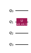
# Prepare the qubit in a state that has coherence and different populations 
initial_state = QuantumCircuit(q)
initial_state.u(np.pi/4, np.pi/4, 0, q[system])
initial_state.draw('mpl')

Tehtävä 3 (4p)

Valmistellaan tilatomografiakoe, jolla analysoimme piirin ja depolarisoivan kohinan tuottamaa tilaa. Tässä rekonstruoimme tiheysmatriisit ja tilojen fideliteetit.

Eri arvoille $p \in [0, 1]$:
1. A) Yhdistä kvanttipiirissä initial_state ja depolarizing_channel.
2. Valmistele ja aja StateTomography, joka löytyy kirjastosta qiskit_experiments.library.tomography tehdäksesi tomografian vain system-kubitille simulaattoria käyttäen.
  - Laske myös fideliteetti verrattuna system-kubitin tilaan initial_state (eli ilman depolarisoivaa kanavaa). Saatat tarvita toimintoa partial_trace qiskit.quantum_info:sta.
  - Laske virherajat fideliteeteille bootstrapping-menetelmällä. Käytä tätä varten StateTomographyAnalysis-kirjastosta qiskit_experiments.library.tomography joillakin argumenteilla ja käytä näitä StateTomography:ssa.
3. Kokoa tiheysmatriisit, fideliteetit ja fideliteettien virheet.
Kuvaile lyhyesti omin sanoin, mitä StateTomography tekee. Mitä täytyy mitata? Miten varmistamme, että tiheysmatriisi on fysiikalinen? (Mahdollisesti hyödyllisiä linkkejä: Quantum State Tomography ja Open Quantum Systems with Qiskit.)

# For example, let's consider 10 equally spaced values of p
p_values = np.linspace(0, 1, 10)

# Here we will create a list of circuits for each different value of p
tomography_circuits = []

for p in p_values:
    circ = initial_state.compose(depolarizing_channel(q, p, system, ancillae))
    tomography_circuits.append(circ)

# Compute fidelities wrt. this state
psi = partial_trace(Statevector(initial_state), [q for q in range(initial_state.num_qubits) if q != system])

# Perform boostrapping for fidelity errors
analysis = StateTomographyAnalysis()
analysis.set_options(target_bootstrap_samples=20)

# Now we perform state tomography in simulation and collect the results
backend = AerSimulator()
# backend = FakeGuadalupe()

# backend = AerSimulator(noise_model=noise_model)
rhos = []
fidelities = []
errors = []
for circ in tomography_circuits:
    st = StateTomography(circ, backend=backend, measurement_indices=[system], analysis=analysis, target=psi)
    data = st.run()
    rhos.append(data.analysis_results('state').value)
    fidelities.append(data.analysis_results('state_fidelity').value.n)
    errors.append(data.analysis_results('state_fidelity').value.s)

Kvanttitilatomografia (StateTomography) mittaa valmistettua tilaa käyttäen tomografisesti täydellistä mittauskantaa. Tulosten avulla voimme rekonstruoida tilan koko tiheysmatriisin. Käyttämällä suoraan näitä tuloksia voidaan kuitenkin saada epäfyysisiä tiloja, joten Qiskit käyttää maksimitodennäköisyyttä löytääkseen fyysisen tiheysmatriisin, joka maksimoi tuloksia vastaavat todennäköisyydet.

Tehtävä 4 (4p)

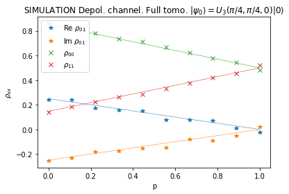
Määritä numeerisesti eksakti tiheysmatriisi system-kubitille depolarisoivan kanavan jälkeen $p$:n funktiona.
Piirrä kuvaajat $\rho_{00}$:n, $\rho_{11}$:n, $\mathrm{Re}(\rho_{01})$:n ja $\mathrm{Im}(\rho_{01})$:n arvoista $p$:n funktiona ja vertaa niitä analyyttisiin ennusteisiin/odotuksiin.
Määritä numeerisesti system-kubitin eksaktit fideliteetit depolarisoivan kanavan jälkeen $p$:n funktiona.
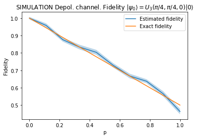
Piirrä kuvaajat system-kubitin eksakteista ja simuloiduista fideliteeteistä verrattuna alkutilaan $p$:n funktiona. Lisää 3. tehtävässä lasketut virherajat kuvaajiin.

Datapisteiden äärellisestä määrästä johtuvia tilastollisia virheitä lukuun ottamatta simulaation tuottamien pisteiden tulisi olla lähellä analyyttistä ennustetta. Fideliteettien osalta virherajat kattavat yhden keskihajonnan (~68 %).

tomo_rhos = np.zeros((2,2,len(p_values)), dtype=complex)

for (i, res) in enumerate(rhos):
    tomo_rhos[:,:,i] = res

# Simulated results
plt.plot(p_values, np.real(tomo_rhos[0,1,:]),"C0*", label='Re $\\rho_{01}$')
plt.plot(p_values, np.imag(tomo_rhos[0,1,:]),"C1*", label='Im $\\rho_{01}$')
plt.plot(p_values, np.real(tomo_rhos[0,0,:]),"C2x", label='$\\rho_{00}$')
plt.plot(p_values, np.real(tomo_rhos[1,1,:]),"C3x", label='$\\rho_{11}$')

# Theoretical prediction

# We obtain the density operator of the initial state
rho0 = partial_trace(Statevector(initial_state), ancillae).data

plt.plot(p_values, np.real(rho0[0,1])*(1-p_values), "C0", linewidth=.5)
plt.plot(p_values, np.imag(rho0[0,1])*(1-p_values), "C1", linewidth=.5)
plt.plot(p_values, 0.5*p_values + np.real(rho0[0,0])*(1-p_values), "C2", linewidth=.5)
plt.plot(p_values, 0.5*p_values + np.real(rho0[1,1])*(1-p_values), "C3", linewidth=.5)

plt.xlabel('p')
plt.ylabel('$\\rho_{xx}$')
plt.legend()

plt.title("SIMULATION Depol. channel. Full tomo. $|\\psi_0\\rangle = U_3(\\pi/4,\\pi/4,0)|0\\rangle$")

Text(0.5, 1.0, 'SIMULATION Depol. channel. Full tomo. $|\\psi_0\\rangle = U_3(\\pi/4,\\pi/4,0)|0\\rangle$')

Tiheysmatriisin alkioiden tarkat lausekkeet depolarisoivan kanavan toiminnalle seuraavat tiheysmatriisille suoritettavasta toiminnasta. Todennäköisyydellä $p$ tila pysyy ennallaan, todennäköisyydellä $(1-p)$ tilaan tulee virhe. Aloitetaan projektissa annetusta kuvauksesta.

$$ \begin{align*} \mathcal{E} (\rho) &= \left[1-\frac 3 4 p \right] \rho + \frac{p}{4} \sum_i \sigma_i \rho \sigma_i \\ &= \left[1-\frac 3 4 p \right] \rho + \frac{p}{4} (\sigma_x \rho \sigma_x + \sigma_y \rho \sigma_y + \sigma_z \rho \sigma_z) \\ &= \left[1- p \right] \rho + \frac{p}{4} (\sigma_0 \rho \sigma_0 + \sigma_x \rho \sigma_x + \sigma_y \rho \sigma_y + \sigma_z \rho \sigma_z) \\ &= \left[1- p \right] \rho + \frac{p}{4} (2 I), \\ \end{align*} $$

jossa viimeinen yhtäsuuruus seuraa tästä: $$ \begin{align*} \sigma_0 \rho \sigma_0 + \sigma_x \rho \sigma_x + \sigma_y \rho \sigma_y + \sigma_z \rho \sigma_z&= \begin{bmatrix} \rho_{00} & \rho_{01} \\ \rho_{10} & \rho_{11} \end{bmatrix}+ \sigma_x \begin{bmatrix} \rho_{00} & \rho_{01} \\ \rho_{10} & \rho_{11} \end{bmatrix} \sigma_x + \sigma_y \begin{bmatrix} \rho_{00} & \rho_{01} \\ \rho_{10} & \rho_{11} \end{bmatrix} \sigma_y + \sigma_z \begin{bmatrix} \rho_{00} & \rho_{01} \\ \rho_{10} & \rho_{11} \end{bmatrix}\sigma_z \\ &= \begin{bmatrix} \rho_{00} & \rho_{01} \\ \rho_{10} & \rho_{11} \end{bmatrix}+\begin{bmatrix} \rho_{11} & \rho_{10} \\ \rho_{01} & \rho_{00} \end{bmatrix}+\begin{bmatrix} \rho_{11} & -\rho_{10} \\ \rho_{01} & \rho_{00} \end{bmatrix} + \begin{bmatrix} \rho_{00} & -\rho_{01} \\ -\rho_{10} & -\rho_{11} \end{bmatrix} \\ &= \begin{bmatrix} 2(\rho_{00} + \rho_{11}) & 0 \\ 0 & 2(\rho_{00} + \rho_{11}) \end{bmatrix} \\ &= 2I, \end{align*} $$ koska tiheysmatriisille pätee $\rho$, $\rho_{00} + \rho_{11} = \mathrm{Tr}[\rho] = 1$.

Siispä depolarisoiva kanava voidaan kirjoittaa: $$\mathcal{E} (\rho) = (1-p) \rho + p \frac{I}{2}$$ Tämä muoto tulee luultavasti useammin vastaan esim. Wikipediassa. Yhden kubitin systeemille nämä ovat yhtäpitävät.

Jos tarkastellaan tiheysmatriisin alkioita kanavan $\rho'$ toiminnan jälkeen, saadaan $$\begin{align*} \rho'_{00} &=(1-p)\rho_{00} + 0.5p \\ \rho'_{11} &=(1-p)\rho_{11} + 0.5p \\ \rho'_{01} &=(1-p)\rho_{01}. \end{align*} $$

# Simulated results
exact_fidelities = []
for circ in tomography_circuits:
    exact_fidelities.append(state_fidelity(psi, partial_trace(DensityMatrix(circ), ancillae)))

plt.plot(p_values, fidelities, "C0", label="Estimated fidelity")
plt.fill_between(p_values, np.array(fidelities) - np.array(errors), np.array(fidelities) + np.array(errors), alpha=.3)
plt.plot(p_values, exact_fidelities, "C1", label="Exact fidelity")

plt.xlabel('p')
plt.ylabel('Fidelity')
plt.legend()

plt.title("SIMULATION Depol. channel. Fidelity $|\\psi_0\\rangle = U_3(\\pi/4,\\pi/4,0)|0\\rangle$")

Text(0.5, 1.0, 'SIMULATION Depol. channel. Fidelity $|\\psi_0\\rangle = U_3(\\pi/4,\\pi/4,0)|0\\rangle$')

Valinnainen lisätehtävä

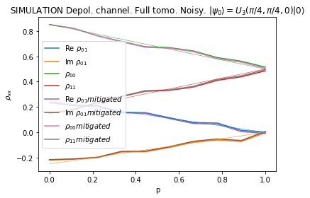
Suorita kaikki yllä olevat tehtävät todellisella laitteella melunvaimennuksen kanssa ja vertaa tuloksia simulaatioon. Tätä varten voit käyttää MitigatedStateTomography:a StateTomography:n sijaan.

Huomaa, että MitigatedTomographyAnalysis toimii hieman eri tavalla kuin StateTomographyAnalysis. Jos tulee ongelmia, kokeile tarjota analyysiluokkaa ajaessasi tomografiakoetta sen sijaan, että teet sen alustaessasi koetta.

Voit hankkia todellisen laitteen taustaohjelman seuraavalla koodilla (primitiivit, kuten Sampler, ovat suhteellisen uusia, joten niitä ei tueta vielä qiskit-experiments-ympäristössä). Varmista lopuksi, että olet luonut ja tallentanut IBM Quantum-tilisi!

# For example, let's consider 10 equally spaced values of p
p_values = np.linspace(0, 1, 10)

# Here we will create a list of circuits for each different value of p
tomography_circuits = []

for p in p_values:
    circ = initial_state.compose(depolarizing_channel(q, p, system, ancillae))
    tomography_circuits.append(circ)

# Compute fidelities wrt. this state
psi = partial_trace(Statevector(initial_state), ancillae)

# Perform boostrapping for fidelity errors
state_tomo = StateTomographyAnalysis()
state_tomo.set_options(target_bootstrap_samples=20)

analysis = MitigatedTomographyAnalysis(tomography_analysis=state_tomo)
analysis.set_options(target=psi, unmitigated_fit=True)

# Now we perform state tomography in simulation and collect the results
backend = FakeGuadalupe()

rhos = []
fidelities = []
errors = []

rhos_mit = []
fidelities_mit = []
errors_mit = []

for circ in tomography_circuits:
    st = MitigatedStateTomography(circ, measurement_indices=[system])
    data = st.run(backend=backend, analysis=analysis)
    rhos_mit.append(data.analysis_results('state')[0].value)
    fidelities_mit.append(data.analysis_results('state_fidelity')[0].value.n)
    errors_mit.append(data.analysis_results('state_fidelity')[0].value.s)
    rhos.append(data.analysis_results('state')[1].value)
    fidelities.append(data.analysis_results('state_fidelity')[1].value.n)
    errors.append(data.analysis_results('state_fidelity')[1].value.s)

Adding a job from a backend (AerSimulator('aer_simulator'
             noise_model=<NoiseModel on ['reset', 'x', 'measure', 'id', 'sx', 'cx']>)) that is different than the current backend (fake_guadalupe). The new backend will be used, but service is not changed if one already exists.
Adding a job from a backend (AerSimulator('aer_simulator'
             noise_model=<NoiseModel on ['reset', 'x', 'measure', 'id', 'sx', 'cx']>)) that is different than the current backend (fake_guadalupe). The new backend will be used, but service is not changed if one already exists.
Adding a job from a backend (AerSimulator('aer_simulator'
             noise_model=<NoiseModel on ['reset', 'x', 'measure', 'id', 'sx', 'cx']>)) that is different than the current backend (fake_guadalupe). The new backend will be used, but service is not changed if one already exists.
Adding a job from a backend (AerSimulator('aer_simulator'
             noise_model=<NoiseModel on ['reset', 'x', 'measure', 'id', 'sx', 'cx']>)) that is different than the current backend (fake_guadalupe). The new backend will be used, but service is not changed if one already exists.
Adding a job from a backend (AerSimulator('aer_simulator'
             noise_model=<NoiseModel on ['reset', 'x', 'measure', 'id', 'sx', 'cx']>)) that is different than the current backend (fake_guadalupe). The new backend will be used, but service is not changed if one already exists.
Adding a job from a backend (AerSimulator('aer_simulator'
             noise_model=<NoiseModel on ['reset', 'x', 'measure', 'id', 'sx', 'cx']>)) that is different than the current backend (fake_guadalupe). The new backend will be used, but service is not changed if one already exists.
Adding a job from a backend (AerSimulator('aer_simulator'
             noise_model=<NoiseModel on ['reset', 'x', 'measure', 'id', 'sx', 'cx']>)) that is different than the current backend (fake_guadalupe). The new backend will be used, but service is not changed if one already exists.
Adding a job from a backend (AerSimulator('aer_simulator'
             noise_model=<NoiseModel on ['reset', 'x', 'measure', 'id', 'sx', 'cx']>)) that is different than the current backend (fake_guadalupe). The new backend will be used, but service is not changed if one already exists.
Adding a job from a backend (AerSimulator('aer_simulator'
             noise_model=<NoiseModel on ['reset', 'x', 'measure', 'id', 'sx', 'cx']>)) that is different than the current backend (fake_guadalupe). The new backend will be used, but service is not changed if one already exists.
Adding a job from a backend (AerSimulator('aer_simulator'
             noise_model=<NoiseModel on ['reset', 'x', 'measure', 'id', 'sx', 'cx']>)) that is different than the current backend (fake_guadalupe). The new backend will be used, but service is not changed if one already exists.

tomo_rhos = np.zeros((2,2,len(p_values)), dtype=complex)

for (i, res) in enumerate(rhos):
    tomo_rhos[:,:,i] = res

tomo_rhos_mit = np.zeros((2,2,len(p_values)), dtype=complex)

for (i, res) in enumerate(rhos_mit):
    tomo_rhos_mit[:,:,i] = res

# Simulated results
plt.plot(p_values, np.real(tomo_rhos[0,1,:]), label='Re $\\rho_{01}$')
plt.plot(p_values, np.imag(tomo_rhos[0,1,:]), label='Im $\\rho_{01}$')
plt.plot(p_values, np.real(tomo_rhos[0,0,:]), label='$\\rho_{00}$')
plt.plot(p_values, np.real(tomo_rhos[1,1,:]), label='$\\rho_{11}$')

plt.plot(p_values, np.real(tomo_rhos_mit[0,1,:]),label='Re $\\rho_{01} mitigated$')
plt.plot(p_values, np.imag(tomo_rhos_mit[0,1,:]), label='Im $\\rho_{01} mitigated$')
plt.plot(p_values, np.real(tomo_rhos_mit[0,0,:]), label='$\\rho_{00} mitigated$')
plt.plot(p_values, np.real(tomo_rhos_mit[1,1,:]), label='$\\rho_{11} mitigated$')

# Theoretical prediction

# We obtain the density operator of the initial state
rho0 = partial_trace(Statevector(initial_state), ancillae).data

plt.plot(p_values, np.real(rho0[0,1])*(1-p_values), "C0", linewidth=.5)
plt.plot(p_values, np.imag(rho0[0,1])*(1-p_values), "C1", linewidth=.5)
plt.plot(p_values, 0.5*p_values + np.real(rho0[0,0])*(1-p_values), "C2", linewidth=.5)
plt.plot(p_values, 0.5*p_values + np.real(rho0[1,1])*(1-p_values), "C3", linewidth=.5)

plt.xlabel('p')
plt.ylabel('$\\rho_{xx}$')
plt.legend()

plt.title("SIMULATION Depol. channel. Full tomo. Noisy. $|\\psi_0\\rangle = U_3(\\pi/4,\\pi/4,0)|0\\rangle$")

Text(0.5, 1.0, 'SIMULATION Depol. channel. Full tomo. Noisy. $|\\psi_0\\rangle = U_3(\\pi/4,\\pi/4,0)|0\\rangle$')

# Simulated results
exact_fidelities = []
for circ in tomography_circuits:
    exact_fidelities.append(state_fidelity(psi, partial_trace(DensityMatrix(circ), ancillae)))

plt.plot(p_values, fidelities, "C0", label="Estimated fidelity")
plt.fill_between(p_values, np.array(fidelities) - np.array(errors), np.array(fidelities) + np.array(errors), alpha=.3)
plt.plot(p_values, fidelities_mit, color="tab:orange", label="Estimated fidelity mitigated")
plt.fill_between(p_values, np.array(fidelities_mit) - np.array(errors_mit), np.array(fidelities_mit) + np.array(errors_mit), color="tab:orange", alpha=.3)
plt.plot(p_values, exact_fidelities, "C1", label="Exact fidelity")

plt.xlabel('p')
plt.ylabel('Fidelity')
plt.legend()

plt.title("SIMULATION Depol. channel. Fidelity. Mitigated. $|\\psi_0\\rangle = U_3(\\pi/4,\\pi/4,0)|0\\rangle$")

Text(0.5, 1.0, 'SIMULATION Depol. channel. Fidelity. Mitigated. $|\\psi_0\\rangle = U_3(\\pi/4,\\pi/4,0)|0\\rangle$')

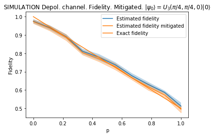
Vaikka lukuvirheen vaimennus auttaa hieman, tulokset eivät vieläkään vastaa odotettuja fideliteetteejä, joten virhelähteitä on oltava muitakin!