
Ratkaisu
# Imports
import numpy as np
import matplotlib.pyplot as plt

# Main qiskit imports
from qiskit import QuantumCircuit, QuantumRegister, ClassicalRegister
from qiskit_aer import AerSimulator
from qiskit_ibm_runtime.fake_provider import FakePerth

# Error mitigation
from qiskit_experiments.library.characterization import LocalReadoutError
# Noisy backend
backend = AerSimulator.from_backend(FakePerth())

# Local simulator
simulator = AerSimulator()
def zz_pump(q, c, p, system, ancilla):
    """Returns a QuantumCircuit implementing the ZZ pump channel on the system qubits

    Args:
        q (QuantumRegister): the register to use for the circuit
        c (ClassicalRegister): the register to use for the measurement of the system qubits
        p (float): the efficiency for the channel, between 0 and 1
        system (list): list of indices for the system qubits
        ancilla (int): index for the ancillary qubit

    Returns:
        A QuantumCircuit object
    """
    zz = QuantumCircuit(q, c)

    theta = 2 * np.arcsin(np.sqrt(p))

    # Map information to ancilla
    zz.cx(q[system[0]], q[system[1]])
    zz.x(q[ancilla])
    zz.cx(q[system][1], q[ancilla])

    # Conditional rotation
    zz.cu(theta, 0.0, 0.0, 0.0, q[ancilla], q[system[1]])

    # Inverse mapping
    zz.cx(q[system[1]], q[ancilla])

    # Measurement
    zz.h(q[system[0]])
    zz.measure(q[system[0]], c[0])
    zz.measure(q[system[1]], c[1])

    return zz
def xx_pump(q, c, p, system, ancilla):
    """Returns a QuantumCircuit implementing the XX pump channel on the system qubits

    Args:
        q (QuantumRegister): the register to use for the circuit
        c (ClassicalRegister): the register to use for the measurement of the system qubits
        p (float): the efficiency for the channel, between 0 and 1
        system (list): list of indices for the system qubits
        ancilla (int): index for the ancillary qubit

    Returns:
        A QuantumCircuit object
    """
    xx = QuantumCircuit(q, c)

    theta = 2 * np.arcsin(np.sqrt(p))

    # Map information to ancilla
    xx.cx(q[system[0]], q[system[1]])
    xx.h(q[system[0]])
    xx.x(q[ancilla])
    xx.cx(q[system[0]], q[ancilla])

    # Conditional rotation
    xx.cu(theta, 0.0, 0.0, 0.0, q[ancilla], q[system[0]])

    # Inverse mapping
    xx.cx(q[system[0]], q[ancilla])

    # Measurement
    xx.measure(q[system[0]], c[0])
    xx.measure(q[system[1]], c[1])

    return xx
def zz_xx_pump(q, c, p, system, ancillae):
    """Returns a QuantumCircuit implementing the composition channel on the system qubits

    Args:
        q (QuantumRegister): the register to use for the circuit
        c (ClassicalRegister): the register to use for the measurement of the system qubits
        p (float): the efficiency for both channels, between 0 and 1
        system (list): list of indices for the system qubits
        ancillae (list): list of indices for the ancillary qubits

    Returns:
        A QuantumCircuit object
    """
    zx = QuantumCircuit(q, c)

    theta = 2 * np.arcsin(np.sqrt(p))

    # ZZ pump
    ## Map information to ancilla
    zx.cx(q[system[0]], q[system[1]])
    zx.x(q[ancillae[0]])
    zx.cx(q[system[1]], q[ancillae[0]])

    ## Conditional rotation
    zx.cu(theta, 0.0, 0.0, 0.0, q[ancillae[0]], q[system[1]])

    ## Inverse mapping
    zx.cx(q[system[1]], q[ancillae[0]])

    # XX pump
    ## Map information to ancilla
    zx.h(q[system[0]])
    zx.x(q[ancillae[1]])
    zx.cx(q[system[0]], q[ancillae[1]])

    ## Conditional rotation
    zx.cu(theta, 0.0, 0.0, 0.0, q[ancillae[1]], q[system[0]])

    ## Inverse mapping
    zx.cx(q[system[0]], q[ancillae[1]])

    # Measurement
    zx.measure(q[system[0]], c[0])
    zx.measure(q[system[1]], c[1])

    return zx
Mukavuden vuoksi määrittelemme funktion, joka palauttaa neljä alkutilan valmistelua
def initial_conditions(q, system):
    """Returns a dictionary containing four QuantumCircuit objects which prepare the two-qubit system in different initial states

    Args:
        q (QuantumRegister): the register to use for the circuit
        system (list): list of indices for the system qubits

    Returns:
        A dictionary with the initial state QuantumCircuit objects and a list of labels
    """
    # State labels
    state_labels = ['00', '01', '10', '11']

    ic = {}
    for ic_label in state_labels:
        ic[ic_label] = QuantumCircuit(q)

    # |01>
    ic['01'].x(q[system[0]])

    # |10>
    ic['10'].x(q[system[1]])

    # |11>
    ic['11'].x(q[system[0]])
    ic['11'].x(q[system[1]])

    return ic, state_labels
SHOTS = 8192

# The values for p
p_values = np.linspace(0, 1, 10)

# We create the quantum circuits
q = QuantumRegister(5, name='q')
c = ClassicalRegister(2, name='c')

## Index of the system qubit
system = [2, 1]

## Indices of the ancillary qubits
a_zz = 0
a_xx = 4

## Prepare the qubits in four initial conditions
ic_circs, ic_state_labels = initial_conditions(q, system)

## Three different channels, each with
## four initial conditions and ten values of p
pumps = ['ZZ', 'XX', 'ZZ_XX']
circuits = {}
for pump in pumps:
    circuits[pump] = {}
    for ic in ic_state_labels:
        circuits[pump][ic] = []
for ic in ic_state_labels:
    for p in p_values:
        circuits['ZZ'][ic].append(ic_circs[ic].compose(zz_pump(q, c, p, system, a_zz)))
        circuits['XX'][ic].append(ic_circs[ic].compose(xx_pump(q, c, p, system, a_xx)))
        circuits['ZZ_XX'][ic].append(ic_circs[ic].compose(zz_xx_pump(q, c, p, system, [a_zz, a_xx])))
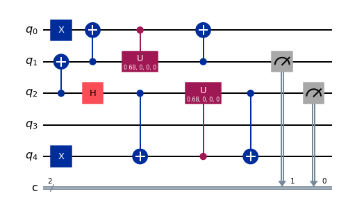
circuits['ZZ_XX']['00'][1].draw(output='mpl')
# Execute the circuits on the local simulator
jobs_sim = {}
for pump in pumps:
    jobs_sim[pump] = {}
    for ic in ic_state_labels:
        jobs_sim[pump][ic] = simulator.run(circuits[pump][ic], shots = SHOTS)

# Analyse the outcomes
overlaps_sim = {}
for pump in pumps:
    overlaps_sim[pump] = {}
    for ic in ic_state_labels:
        overlaps_sim[pump][ic] = [0.0]*len(p_values)
    for i in range(len(p_values)):
        for ic in ic_state_labels:
            counts = jobs_sim[pump][ic].result().get_counts(i)
            for outcome in counts:
                overlaps_sim[pump][outcome][i] += counts[outcome]/(4.0 * float(SHOTS))

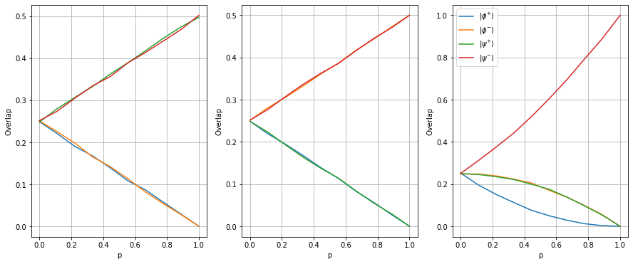
# Plot the results
fig_idx = 131
plt.figure(figsize=(15,6))
bell_labels = {'00': r"$| \phi^{+} \rangle$", '01': r"$| \phi^{-} \rangle$", '10': r"$| \psi^{+} \rangle$", '11': r"$| \psi^{-} \rangle$"}
for pump in pumps:
    plt.subplot(fig_idx)
    for outcome in overlaps_sim[pump]:
        plt.plot(p_values, overlaps_sim[pump][outcome], label = bell_labels[outcome])
    plt.xlabel('p')
    plt.ylabel('Overlap')
    fig_idx += 1
    plt.grid()
plt.legend()
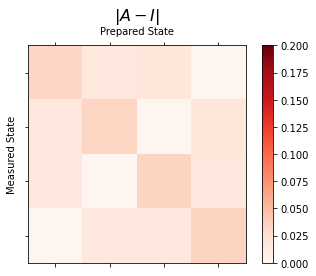
exp = LocalReadoutError(system, backend=backend)
exp.analysis.set_options(plot=True)
res = exp.run(shots=SHOTS)
mitigator = res.analysis_results(0).value
res.figure(0)
# Execute the circuits on the local simulator
jobs_sim = {}
for pump in pumps:
    jobs_sim[pump] = {}
    for ic in ic_state_labels:
        jobs_sim[pump][ic] = backend.run(circuits[pump][ic], shots = SHOTS)

overlaps = {}
overlaps_mit = {}

for pump in pumps:
    overlaps[pump] = {}
    overlaps_mit[pump] = {}
    for ic in ic_state_labels:
        overlaps[pump][ic] = [0.0]*len(p_values)
        overlaps_mit[pump][ic] = [0.0]*len(p_values)
    for i in range(len(p_values)):
        for ic in ic_state_labels:
            counts = jobs_sim[pump][ic].result().get_counts(i)
            unmitigated_probs = {label: count / SHOTS for label, count in counts.items()}
            mitigated_quasi_probs = mitigator.quasi_probabilities(unmitigated_probs)
            mitigated_probs = mitigated_quasi_probs.nearest_probability_distribution().binary_probabilities()
            for outcome in unmitigated_probs:
                overlaps[pump][outcome][i] += unmitigated_probs[outcome]/4
            for outcome in mitigated_probs:
                overlaps_mit[pump][outcome[::-1]][i] += mitigated_probs[outcome]/4

# Plot the results
fig_idx = 131
plt.figure(figsize=(15,6))
colors = plt.rcParams['axes.prop_cycle'][0:4]
cycler_2 = plt.cycler(color=colors)
bell_labels = {'00': r"$| \phi^{+} \rangle$", '01': r"$| \phi^{-} \rangle$", '10': r"$| \psi^{+} \rangle$", '11': r"$| \psi^{-} \rangle$"}
for pump in pumps:
    plt.subplot(fig_idx)
    plt.gca().set_prop_cycle(cycler_2)
    for outcome in overlaps[pump]:
        plt.plot(p_values, overlaps[pump][outcome], label = f"{bell_labels[outcome]} noisy", ls='--')
    for outcome in overlaps_mit[pump]:
        plt.plot(p_values, overlaps_mit[pump][outcome], label = f"{bell_labels[outcome]} mitigated")
    plt.xlabel('p')
    plt.ylabel('Overlap')
    fig_idx += 1
    plt.grid()
plt.legend()
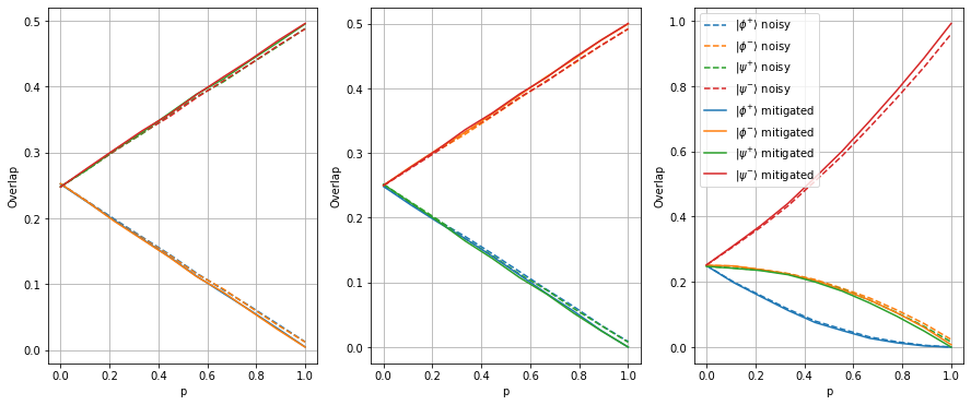
Ero vaimennetun ja vaimentamattoman lukuvirheen välillä ei ole kovin suuri, koska mittaamme tässä vain kahta kubittia. Mutta mitä enemmän kubitteja on, sitä enemmän virheet kasautuvat ja sitä tärkeämmäksi lukuvirheen vaimennus tulee!